Simulating thousands of birds without feathers flocking together
Reviewing the bird-physics literature and building a tunable simulation of the collective motion of a flock
A few thousand birds can turn together, stretch into a ribbon, or divide around an obstacle without anyone appearing to direct traffic.
One way to animate a flock is to decide where every bird should go and draw the paths. Craig Reynolds took a different approach in his 1987 paper on boids. He gave simulated individuals local behaviors: avoid crowding, align with nearby individuals, and stay near the group. The flock’s motion followed from repeatedly applying those rules. As his abstract puts it, the birds (or equivalently boids for New Yorkers) “choose their own course” (Reynolds, 1987).
That is a useful start, but it leaves a lot unspecified. What counts as nearby? Do birds align their directions or their full velocities? How do those local interactions let a flock change direction and stay together?
Birds are not a gas at equilibrium (and flocks cannot be approximated as a sphere for that matter)
The connection to statistical physics is fairly direct. We have many interacting degrees of freedom, local fluctuations, and a collective state. But birds continually consume energy to move. Their speed does not simply decay by drag until everything comes to rest. They are examples of active matter: the constituents take in energy and convert it into motion or mechanical work (Ramaswamy, 2010).
These systems, as you can imagine, don't gradually settle to equilibrium. For birds, dissipation includes energy transferred to the air and heat. Flocks of birds form these familiar collective swarms. Walk under a flock and you may find out what else they dissipate on your freshly washed clothes.
In the model introduced by Vicsek and collaborators in 1995, particles move at a fixed speed and update their headings toward the local average, with added directional noise. There is no leader supplying the direction of travel. Nevertheless, coordinated motion can emerge (Vicsek et al., 1995). This simplified mechanic lets us ask about ordering without first determining the biomechanics of a wing, much as we can predict the orbit of a planet without worrying so much about how matter is distributed within it.
A convenient measure of directional order is the polarization,
where is the unit vector along bird ’s velocity and is the number of birds. If all headings agree, . If headings largely cancel, is small. However, this does not tell us everything. An organized flock moving around a circle can have a small total polarization.
Toner and Tu instead described slowly varying density and velocity fields. Their 1995 continuum equations are
Here is number density, is the coarse-grained velocity, and is random forcing. The density-dependent pressure is written here to distinguish it from polarization. The terms select a nonzero speed when , the terms smooth spatial variations, and the second equation conserves bird number (Toner and Tu, 1995).
The convective term carries orientation as the individuals move and exchange neighbors. Their analysis finds stable orientational order even in two dimensions. A moving state selects a direction although the equations select none: spontaneous symmetry breaking away from equilibrium. The equilibrium Mermin–Wagner restriction therefore does not decide this problem. The conclusion depends on the nonlinear dynamics, not just the uniform solution (Toner and Tu, 1995).
Seven neighbors seven meters
Suppose every bird responds to all other birds within a fixed radius. Compress the flock and the number of interaction partners increases. Let it spread out and that number decreases; eventually some birds lose contact altogether. This is a metric neighborhood,
It selects the other birds whose positions lie inside an open ball in the language of metric spaces. In flocking, a topological neighborhood usually means a fixed number of nearest individuals. Their distances change as the flock expands, but their number does not. This specialized usage is about neighbor rank. “The seventh closest bird” is a different instruction from “every bird within seven meters.”
Ballerini and company used three-dimensional reconstructions of starling flocks to investigate this distinction. They inferred an interaction range from the anisotropy of neighbor positions: nearby birds were not distributed uniformly around a reference bird, and that directional structure weakened with increasing neighbor rank. Across flocks with different densities, their results supported roughly six or seven* neighbors rather than a constant distance (Ballerini et al., 2008).
* A notable pair of numbers in these modern times

The inference of seven comes from spatial structure and is experimentally motivated as a starting point; it does not directly record which birds each individual was watching. Let's bring that into our working model.
There is also no reason to make every interaction topological. Two bodies can collide whether they are each other’s first or twentieth neighbor. The model for this article uses nearest-neighbor selection for social coordination and a separate distance-dependent rule for close encounters.
Try changing the neighbor count while leaving the other settings alone. Increasing it changes which information each bird averages. That doesn't guarantee a more responsive flock, as averaging over more individuals may also dilute a local changes.
What starts a turnaround?
The original version of this animation had a straightforward problem: strong alignment, weak individual fluctuations, and no horizontal environmental preference. Adding a bird leading the pack on a prescribed route would create turns, but would also supply much of the answer in advance.
In a study of spontaneous turns, Attanasi and collaborators found initiators near the flock’s outer tips (Attanasi et al., 2015).
For the scene here, I have added a preference to remain near a roost. Hildenbrandt, Carere, and Hemelrijk’s StarDisplay combines local coordination with simplified flight mechanics and attraction toward a roosting region. Its horizontal return response depends on the bird’s heading: stronger when flying outward, weaker when already returning (Hildenbrandt et al., 2010).
Our birds similarly turn back after leaving a region, then continue inward before releasing that preference. They respond individually and influence their neighbors through the social terms discussed in What the simulation does.
How far does a turn travel?
A flock can have high polarization and still respond badly when something happens. Everyone might be traveling in the same direction, yet a turn by a few individuals could be lost before it reaches the rest. Photos of starling flocks alone don't settle this question.
In 2010, Cavagna and collaborators measured correlations between velocity fluctuations in starling flocks. The range of those correlations grew with the flock’s linear size. This is the sense in which the correlations were called scale free, meaning they did not reveal a fixed correlation length independent of the size of the group (Cavagna et al., 2010).
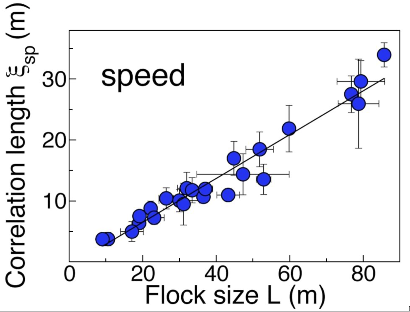
A bird can interact directly with a few neighbors while sharing correlated fluctuations with birds much farther away. You might interact regularly with a small group of friends and share tastes with a much wider circle. But by the time you get to Kevin Bacon (see Six Degrees of Kevin Bacon), there likely isn't much in common. Interaction range correlation length.
The distinction is made clear during a turn. Attanasi and collaborators reconstructed turning starling flocks and found directional information propagating with a “linear dispersion law and negligible attenuation.” Their theory introduced behavioral inertia: resistance to changing the curvature of a flight path. In the nearly planar, ordered limit, their equations (6) and (8) read (Attanasi et al., 2014)
Here is the heading angle, is its conjugate spin variable, is behavioral inertia, is the average nearest-neighbor spacing, and is the theory’s alignment stiffness. These are the paper’s variables, not numerical values taken from our sliders. The resulting wave equation carries a turn with speed .
In our simulation, matching velocities and copying a turn after a delay can produce a collective turn. To compare it with these experiments, we would also need to measure how quickly the turn spreads and how much it weakens.
Why a flock darkens and divides
A bird presents a different silhouette when it banks. If nearby birds copy that maneuver, a dark band can travel through the flock without an equally large change in density. Hemelrijk and collaborators reproduced this effect with rolling maneuvers in a model of agitation waves (Hemelrijk et al., 2015). A two-dimensional view can also make birds at different heights appear to pass through one another.
Banking changes more than the view. Tilting the lift force makes some of it available for turning and leaves less to oppose gravity. Unless the bird increases lift, it loses height. In StarDisplay, coupling turns to flight mechanics helped produce changing flock shapes (Hemelrijk and Hildenbrandt, 2011). Our birds now have a bank angle and a lift response that affect their trajectories, rather than only tilting a mesh after the turn has happened.
The 50,000- and 100,000-point modes retain the movement rules but cannot display that wing-area effect. Wingbeats are just an animation and do not contribute in any aerodynamic way.
A split doesn't have to divide the flock in half. Papadopoulou and collaborators studied flocks pursued by a robotic falcon: different birds turned or dived at different times, and some groups separated while others remained connected (Papadopoulou et al., 2026). Those observations concern escape behavior.
Occasional disturbances arise near the flock’s edge. Affected birds briefly prioritize a turn or dive, and neighbors can copy it after a delay. The response weakens as it spreads. Neither the number of resulting groups nor their sizes is specified. Once the maneuver ends, normal coordination returns; groups can join again when their paths bring them close. The disturbance’s cause is not simulated.
What the simulation does
The equations below specify an effective steering model. Its constants, response times and limits are implementation choices, not fitted measurements.
Bird has position , velocity , and heading . Its target acceleration, , is the sum of the responses below. Distances are in meters and time is in seconds.
The small diagrams isolate individual terms and have their own controls.
1. Choose the neighbors
is the set of the nearest birds. A bar is their average: for example, . If fewer than candidates are available, the average uses that smaller number. An empty set contributes no social attraction or alignment.
Below 20,000 birds, a spatial tree organizes the birds by their positions in three-dimensional space. It finds the nearest 24 birds without comparing every possible pair; the first contribute to the social coordination term.
2. Match velocity and stay together
The first term reduces differences in speed and direction. Its strength has units . The second pulls toward the neighbors’ average position, with in . Increasing the neighbor count changes the information available to the bird. Increasing these strengths makes it respond more strongly to that information.
3. Leave room for wings
contains nearby candidates within the personal-space radius . Repulsion acts along the line between the two birds and decreases linearly to zero at . Here . Repulsion is evaluated for up to 24 candidates.
4. Return toward the roost
Local cohesion keeps neighbors together; the roost response gives them a place to return to. A bird starts returning after leaving radius and continues until it reaches .
is 1 during a return and 0 otherwise. is the horizontal heading, points horizontally from the roost to the bird, and points sideways. The dot products set the turn’s direction and strength; the hyperbolic tangent limits the command. The roost slider sets in acceleration units. At zero, horizontal flight is unrestricted.
5. Choose altitude and individual variation
has only a vertical component. It strengthens when the predicted height two seconds ahead falls below 11 meters or above 34 meters, with a weaker preference for 20 meters. The remaining term, , gives each bird a smoothly changing individual preference.
Altitude and noise equations
Here is one component of the current individual acceleration preference, and is its value after the next perception update. Each component follows this update independently. is the elapsed time between perception updates, is a seeded standard normal sample, and sets the long-time standard deviation of each component. The exponential factor retains some of the preceding preference over correlation time .
6. Respond to a local disturbance
The disturbance response is a temporary preference of direction. A patch near the flock’s edge receives a shared turn command, sometimes accompanied by a dive.
Each pulse starts at , has amplitude , and lasts . Here chooses the turn direction and sets the downward component. Alignment and cohesion are multiplied by during the maneuver; separation and environmental responses remain active.
An eligible bird copies the strongest active maneuver among its social neighbors after a delay, with reduced amplitude. The response weakens as it spreads.
Putting those responses together gives the bird equation shown in the controls:
Details about implementation
A bird cannot instantly adopt the entire requested acceleration. First separate the turning part from the part that changes speed. The matrix removes the component along the heading; is the identity matrix. Define for a nonzero vector, and zero for a zero vector. This limits its length without changing its direction.
is the limited turning target, is the stored steering acceleration, and superscript labels the current step. Over one step , steering moves partway toward the target. The slider controls how gradually it responds.
Banking changes the flight path
Let point sideways and point upward perpendicular to the heading. The stored steering projected onto these directions gives requests and . A reduced pitch controller limits the upward request to keep ordinary flight away from vertical aerobatics:
Angles are in radians. With and , the requested bank and lift per unit mass are
The actual bank and specific lift relax toward these requests by the same exponential update used above. The response time is 0.22 seconds when rolling farther into a bank, 0.44 seconds when rolling out, and 0.65 seconds for lift. Because lift lags behind banking, a turn can initially lose height. The resulting turning acceleration is
This resolves lift and the perpendicular component of gravity. The speed controller below stands in for propulsion and drag, including compensation for gravity along the heading. This is not a complete aerodynamic model.
changes speed along the heading. The first contribution relaxes speed toward the preferred value ; the second preserves the forward social response, so a bird can slow behind another or catch up. The clip operation limits this acceleration to the interval shown.
Before advancing position, the candidate velocity is rescaled to the intended speed . Its total change from the preceding velocity is then limited to , with . That final limit also applies after a slider change. This discrete rule defines the browser model.
Roost and initial conditions
The default roost radius is
Here sets the initial cloud’s size. The roost center is ; the cloud begins near , avoiding a symmetric launch directly away from the center. An exactly radial heading uses a small seeded left-or-right choice to break the tie. The return memory and smooth turn command are inspired by StarDisplay’s heading-dependent roost attraction.
Disturbance timing
The first disturbance occurs after five simulated seconds; subsequent intervals are chosen uniformly between 40 and 60 seconds. A randomly oriented edge of the flock receives the disturbance within radius .
Initial pulse amplitudes range from 0.75 to 1, and durations from 2.8 to 3.6 seconds. Some events include a dive whose strength varies with position within the affected patch. Copying introduces a delay of 0.12–0.28 seconds and retains 96% of the donor’s amplitude, stopping below amplitude 0.25. A bird responds at most once to the same disturbance, then waits five seconds after its maneuver before responding to another. Pending responses cannot propagate until their start time, so updating birds in an array does not transmit a disturbance instantly.
The shortcut for large flocks
At 20,000, 50,000, and 100,000 individuals, three-meter grid cells replace the tree. The search examines at most 64 candidates from 27 adjacent cells, with at most 12 from any one cell. The nearest 24 of those candidates supply the same force terms. They don't need to be the globally nearest birds. This is my spherical cow for your computer’s sake.
Perception updates every two physics steps below 10,000 birds, every four at 10,000 and 20,000, and every ten at 50,000 and 100,000. From 10,000 birds upward, this work is staggered across birds, while all positions and velocities advance at 30 Hz in simulation time. Noise uses the corresponding elapsed perception time. Because the search, sampling interval, and roost size vary, these modes are not all-else-controlled-for finite-size comparisons.
Playback runs at 1.5× speed: one second on screen advances the model by 1.5 seconds. The fixed timestep and all physical parameters stay the same; the worker performs more steps per second of wall-clock time.
The update loop
Every target uses the same old positions and velocities; a disturbance copied in this pass starts in the future. Otherwise, birds later in the loop would effectively see into the future.
every 1/30 second of simulation time (1.5x playback):
    update local disturbance pulses and any new disturbance
    on a perception step:
        organize current positions for the neighbor search
        for each bird due to update its perception:
            find up to 24 nearby candidates
            average the nearest k positions and velocities
            schedule delayed copying of a nearby maneuver, if eligible
            reduce social response during escape; add its turn/dive command
            add repulsion from candidates within personal space
            update its return-to-roost state
            add roost turning, altitude response, and correlated noise
            store the target acceleration

    for each bird, using the same previous state:
        separate target acceleration into sideways and forward parts
        limit the sideways target and gradually adjust stored steering
        update bank angle and lift toward the steering request
        resolve lift and gravity to obtain turning acceleration
        combine the forward target with preferred-speed regulation
        update velocity, limiting speed and total velocity change

    for each bird:
        advance position with its new velocity
    send a snapshot to the display

while the panel is visible and playing, up to 120 frames per second:
    interpolate between completed simulation states on the GPU
    follow the flock with the camera
draw shared bird meshes, or small points for 50,000 and aboveBoth the drawing and physics pause while the simulation is offscreen, so reading about birds gives the computer a rest.
And, because there are technically no feathers on our bird…
Behold! Plato’s Man!
This here sparrow has a 24-centimeter wingspan and is made of 882 triangles. It was made with OpenAI’s GPT-6 Astra using the Computer Use tool in Blender, before I learned of the obsession the bird-watching physicists have with the starling.
As you can see by starting its wingbeat, this poor featherless bird's skull deforms with every never-ending flap of its wings. And with a few thousand more, we have our flock.
References & further reading
- Alessandro Attanasi et al. (2014). Information transfer and behavioural inertia in starling flocks. Nature Physics 10, 691–696. doi: 10.1038/nphys3035.
- Alessandro Attanasi et al. (2015). Emergence of collective changes in travel direction of starling flocks from individual birds’ fluctuations. Journal of the Royal Society Interface 12, 20150319. doi: 10.1098/rsif.2015.0319.
- M. Ballerini et al. (2008). Interaction ruling animal collective behavior depends on topological rather than metric distance: Evidence from a field study. Proceedings of the National Academy of Sciences 105, 1232–1237. doi: 10.1073/pnas.0711437105.
Open author preprint; journal title and citation follow the published version.
- Clemens Bechinger et al. (2016). Active Particles in Complex and Crowded Environments. Reviews of Modern Physics 88, 045006. doi: 10.1103/RevModPhys.88.045006.
- Andrea Cavagna, Alessio Cimarelli, Irene Giardina, Giorgio Parisi, Raffaele Santagati, Fabio Stefanini, and Massimiliano Viale (2010). Scale-free correlations in starling flocks. Proceedings of the National Academy of Sciences 107, 11865–11870. doi: 10.1073/pnas.1005766107.
- Charlotte K. Hemelrijk and Hanno Hildenbrandt (2011). Some Causes of the Variable Shape of Flocks of Birds. PLOS ONE 6(8), e22479. doi: 10.1371/journal.pone.0022479.
- Charlotte K. Hemelrijk, Lars van Zuidam, and Hanno Hildenbrandt (2015). What underlies waves of agitation in starling flocks. Behavioral Ecology and Sociobiology 69, 755–764. doi: 10.1007/s00265-015-1891-3.
- H. Hildenbrandt, C. Carere, and C. K. Hemelrijk (2010). Self-organized aerial displays of thousands of starlings: A model. Behavioral Ecology 21(6), 1349–1359. doi: 10.1093/beheco/arq149.
The university record includes the published PDF.
- M. C. Marchetti et al. (2013). Hydrodynamics of soft active matter. Reviews of Modern Physics 85, 1143–1189. doi: 10.1103/RevModPhys.85.1143.
- Marina Papadopoulou, Hanno Hildenbrandt, Rolf F. Storms, Claudio Carere, Simon Verhulst, and Charlotte K. Hemelrijk (2026). A mechanistic understanding of collective escape in starling flocks. Communications Biology 9, 1055. doi: 10.1038/s42003-026-10173-4.
- Sriram Ramaswamy (2010). The Mechanics and Statistics of Active Matter. Annual Review of Condensed Matter Physics 1, 323–345. doi: 10.1146/annurev-conmatphys-070909-104101.
- Craig W. Reynolds (1987). Flocks, Herds, and Schools: A Distributed Behavioral Model. Computer Graphics 21(4), 25–34.
The author’s paper page, with links to the full text.
- John Toner and Yuhai Tu (1995). Long-Range Order in a Two-Dimensional Dynamical XY Model: How Birds Fly Together. Physical Review Letters 75, 4326–4329. doi: 10.1103/PhysRevLett.75.4326.
- Tamás Vicsek, András Czirók, Eshel Ben-Jacob, Inon Cohen, and Ofer Shochet (1995). Novel Type of Phase Transition in a System of Self-Driven Particles. Physical Review Letters 75, 1226–1229. doi: 10.1103/PhysRevLett.75.1226.
Author-deposited copy of the 1995 paper; the arXiv deposit is dated 2006.
Related simulations
- Max Comstock (2023). Simulating the Dynamics of Large Flocks of Birds. SIAM News. A browser simulation using WebGL and model predictive control.
- Alex Scott. Murmuration. An interactive flocking project with two- and three-dimensional views and tunable local behavior.